Univariate Interpolation Examples in Python (part-1)

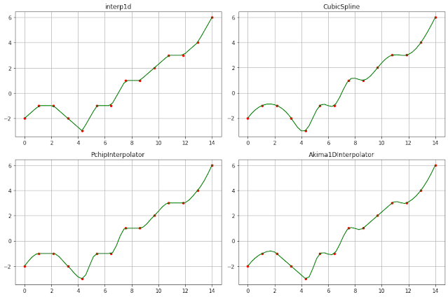
     Interpolation is a technique used to estimate unknown data points within a known range, aiming to create a smoother curve. Univariate interpolation specifically focuses on fitting a curve to a set of two-dimensional data points sampled from a single-variable function. This process enhances the continuity of the curve within the given range.

     SciPy API provides several functions to implement the interpolation method for a given data. In this tutorial, you'll learn how to apply interpolation for a given data by using interp1d, CubicSpline, PchipInterpolator, and Akima1DInterplator methods in Python. The tutorial covers;

1. Preparing test data
   
2. 1-D interpolation with interp1d
3. CubicSpline method
4. PchipInterpolator  method
5. Akima1DInterpolator method
   
6. Source code listing
   

    We'll start by loading the required libraries.

from scipy import interpolate
import matplotlib.pyplot as plt
import numpy as np 

Preparing test data

 

   We'll create a simple x and y data for this tutorial. We can visualize it on a graph and apply linear interpolation. Linear interpolation in a graph is simply connecting data points linearly.

 

y = [-2,-1,-1,-2,-3,-1,-1, 1, 1, 2, 3, 3, 4, 6]
x = np.linspace(0, len(y), len(y))

plt.plot(x, y, '.r', markersize=10)

plt.plot(x, y)

plt.grid()        
plt.show() 

 

 

1-D interpolation with interp1d

    An interp1d class finds the value of new points of one-dimensional function with a given method such as linear, nearest, cubic, and etc. The below listing shows implementation of interp1d method. First, we'll fit model on x and y data, then provide new x data to find out new estimated y values.

xnew = np.linspace(min(x), max(x), num=50)
oned = interpolate.interp1d(x, y)
yfit = oned(xnew)

plt.plot(x, y, '.')
plt.plot(xnew, yfit)
plt.grid()
plt.show() 

 

CubicSpline method

    CubicSpline uses a piecewise cubic polynomial that is twice continuously differentiable to interpolate data. The implementation of CubicSpline method is similar to above scripting. 

 
oned = interpolate.CubicSpline(x, y)
yfit = oned(xnew)

plt.plot(x, y, '.')
plt.plot(xnew, yfit)
plt.grid()
plt.show() 

   

PchipInterpolator method

    PCHIP (Piecewise Cubic Hermite Interpolating Polynomial) 1-D monotonic cubic interpolation employs monotonic cubic splines to determine the value of new points. The implementation of PchipInterpolator method is also similar to above scripting.

pchip = interpolate.PchipInterpolator(x, y)
yfit = pchip(xnew)

plt.plot(x, y, '.')
plt.plot(xnew, yfit)
plt.grid()
plt.show() 

 

 

Akima1DInterpolator method

    Akima1DInterpolator fits piecewise cubic polynomials. Akima's interpolation method employs a continuously differentiable sub-spline constructed from piecewise cubic polynomials. The implementation of Akima1DInterpolator method is shown below.

akima = interpolate.Akima1DInterpolator(x, y)
yfit = akima(xnew)

plt.plot(x, y, '.')
plt.plot(xnew, yfit)
plt.grid()
plt.show() 

 

    Finally, we put all together in one graph and compare each method performance with a given data. The following listing shows how to plot all in one graph.

# fit each method on x, y data 

oned = interpolate.interp1d(x, y)
akima = interpolate.Akima1DInterpolator(x, y)
cubic = interpolate.CubicSpline(x, y)
pchip = interpolate.PchipInterpolator(x, y)

# create dictionary 
funcs = {
    oned:"interp1d",
    cubic:"CubicSpline",
    pchip:"PchipInterpolator",
    akima:"Akima1DInterpolator" } 

# visualize in a graph

i = 0
ig, ax = plt.subplots(nrows=2, ncols=2, figsize=(12, 8))
for row in range(2):
    for col in range(2):
        ax[row][col].plot(x, y, '.', c="g", markersize=8)
        yfit = list(funcs.keys())[i](xnew)
        ax[row][col].plot(xnew, yfit, 'r')
        ax[row][col].set_title(list(funcs.values())[i])
        ax[row][col].grid()
        i = i + 1
        
plt.tight_layout()        
plt.show()  

  

 

    In this tutorial, we've briefly learned how to interpolate data by using SciPy's interp1d, CubicSpline, PchipInterpolator, and Akima1DInterplator classes in Python. The full source code is listed below. 

 

 

Source code listing

from scipy import interpolate
import matplotlib.pyplot as plt
import numpy as np

# Preparing data

y = [-2,-1,-1,-2,-3,-1,-1, 1, 1, 2, 3, 3, 4, 6]
x = np.linspace(0, len(y), len(y))

plt.plot(x, y, '.r', markersize=10)

plt.plot(x, y)

plt.grid()        
plt.show() 

xnew = np.linspace(min(x), max(x), num=50)

# interp1d interpolation 
oned = interpolate.interp1d(x, y)
yfit = oned(xnew)

plt.plot(x, y, '.')
plt.plot(xnew, yfit)
plt.grid()
plt.show() 

# CubicSpline interpolation 
cubic = interpolate.CubicSpline(x, y)
yfit = cubic(xnew)

plt.plot(x, y, '.')
plt.plot(xnew, yfit)
plt.grid()
plt.show() 

# PchipInterpolator interpolation 
pchip = interpolate.PchipInterpolator(x, y)
yfit = pchip(xnew)

plt.plot(x, y, '.')
plt.plot(xnew, yfit)
plt.grid()
plt.show()

# Akiam1DInterpolator interpolation 
akima = interpolate.Akima1DInterpolator(x, y)
yfit = akima(xnew)

plt.plot(x, y, '.')
plt.plot(xnew, yfit)
plt.grid()
plt.show()  

# fit each method on x, y data 
oned = interpolate.interp1d(x, y)
akima = interpolate.Akima1DInterpolator(x, y)
cubic = interpolate.CubicSpline(x, y)
pchip = interpolate.PchipInterpolator(x, y)

# create dictionary 
funcs = {
    oned:"interp1d",
    cubic:"CubicSpline",
    pchip:"PchipInterpolator",
    akima:"Akima1DInterpolator" }   

# visualize in a graph  

i = 0
ig, ax = plt.subplots(nrows=2, ncols=2, figsize=(12, 8))
for row in range(2):
    for col in range(2):
        ax[row][col].plot(x, y, '.', c="g", markersize=8)
        yfit = list(funcs.keys())[i](xnew)
        ax[row][col].plot(xnew, yfit, 'r')
        ax[row][col].set_title(list(funcs.values())[i])
        ax[row][col].grid()
        i = i + 1
        
plt.tight_layout()        
plt.show()

 

References:

1. SciPy Interpolation