Fourier Transform Example with SciPy Functions

    A Fourier transform is a method to decompose signal data in a frequency components. By using this function, we can transform a time domain signal into the frequency domain one and a vice versa. It is widely used in signal processing and many other applications. 

    Discrete Fourier Transform (DFT) is an algorithm to transform a discrete (finite-duration) signal data. Fast Fourier Transform (FFT) is an efficient algorithm that implements DFT. 

    SciPy API provides several functions to implement Fourier transform.  

    In this tutorial, we'll briefly learn how to transform and inverse transform a signal data by SciPy API functions. The tutorial covers:

1. Preparing the data
2. Transform with fft()
   
3. Transform with rfft()
4. Inverse transform
   
5. Source code listing

   We'll start by loading the required libraries for this tutorial.

import numpy as np
import matplotlib.pyplot as plt
from sklearn.preprocessing import normalize
from scipy.fft import fft, fftfreq
from scipy.fft import rfft, rfftfreq
from scipy.fft import irfft 

Preparing the data

   First, we'll generate sample data for this tutorial. Here, we define frequency, duration, and sampling rate to generate sequence data.

 

frequency = 3
duration = 2
sampling_rate = 2000
N = sampling_rate * duration 

Next, we'll generate x and y data by using above definitions and visualize it in a plot. We can add some noise or the data with different frequency into the y.

 

x = np.linspace(0, duration, N, endpoint = False)
frequencies = x * frequency

y = np.sin((2 * np.pi) * x * frequency)

noise = np.random.normal(0, 1, size = len(x))
y = y + noise * 0.1 

plt.plot(x, y)
plt.show()

 

 

 

In a next step we'll normalize y data.

normalized_y = normalize(y[:,np.newaxis], axis=0).ravel()

plt.plot(x, normalized_y)
plt.show()

Transform with fft()

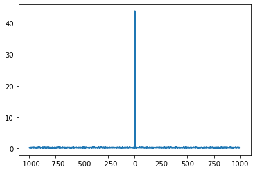
   To transform prepared data, we use fft() and freqfft() function of SciPy API. The fft() function returns discrete Fourier transform of real or complex sequence and the fftfreq() returns the discrete Fourier transform sample frequencies.

ffty = fft(normalized_y)
fftx = fftfreq(N, 1 / sampling_rate)

plt.plot(fftx, np.abs(ffty))
plt.show() 

 

Transform with rfft()

    The rfft() function transforms real sequence sample data and it runs faster than fft().

rffty = rfft(normalized_y)
rfftx = rfftfreq(N, 1 / sampling_rate)

plt.plot(rfftx, np.abs(rffty))
plt.show()  

 

    As you've noticed, the negative part of the output data will be eliminated in this transform.

 

Inverse FFT

 

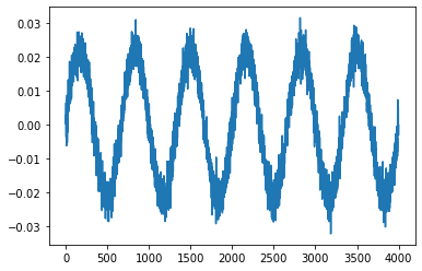
    We can transform back from the fft() output data by using irfft() function.

invers_y = irfft(rffty)

plt.plot(invers_y)
plt.show()

 

 

   In this tutorial, we've briefly learned how to implement Fourier transform for a given signal data and by using SciPy function. The full source code is listed below.

Source code listing

 

import numpy as np
import matplotlib.pyplot as plt
from sklearn.preprocessing import normalize
from scipy.fft import fft, fftfreq
from scipy.fft import rfft, rfftfreq
from scipy.fft import irfft


frequency = 3
duration = 2
sampling_rate=2000 

N = sampling_rate * duration

x = np.linspace(0, duration, N, endpoint=False)

y = np.sin((2 * np.pi) * x * frequency)
plt.plot(x, y)
plt.show()

noise = np.random.normal(0, 1, size=len(x))
y = y + noise*0.1

plt.plot(x, y)
plt.show()

normalized_y = normalize(y[:,np.newaxis], axis=0).ravel()

plt.plot(x, normalized_y)
plt.show()

ffty = fft(normalized_y)
fftx = fftfreq(N, 1 / sampling_rate)

plt.plot(fftx, np.abs(ffty))
plt.show()

rffty = rfft(normalized_y)
rfftx = rfftfreq(N, 1 / sampling_rate)

plt.plot(rfftx, np.abs(rffty))
plt.show()

invers_y = irfft(rffty)

plt.plot(invers_y)
plt.show() 

References:

1. SciPy Fourier Transforms